Modal analysis
Natural frequencies and mode shapes — mass modelling, participation factors and what the numbers are good for.
Analysis types 5 min read
Modal analysis finds the natural frequencies and mode shapes of the structure by solving the generalised eigenvalue problem
where is the stiffness matrix, the mass matrix, a natural circular frequency and its mode shape. The frequency and period engineers quote follow from :
What it needs that static analysis does not
Mass. A static model can be correct with only stiffness defined; a modal model cannot. Mass reaches the analysis from exactly three places, and they add:
- The structure itself — on members and on plates, derived from the materials already in the model.
- Masses you place — a point mass or a rotary inertia at a node, or a mass running along a member. Non-structural mass goes here: cladding, plant, a tank of water.
- Load cases you convert — a mass group naming the cases to turn into mass, and the fraction of each to take. This is where on the imposed load belongs.
A load is not a mass. Elementarium never infers one from the other: a force and the mass that would produce it are independent statements, and deriving one from the other is a guess about gravity. The conversion in (3) is explicit so that its rules can be argued with.
Consistent or lumped
The mass matrix can be consistent (distributed with the element's own interpolation) or lumped onto the diagonal. Consistent mass bounds the true frequencies from above; lumped mass usually lands below them, though that is not guaranteed. Consistent is the default, being the more accurate for the same number of degrees of freedom. Solving both and comparing is a cheap sanity check on a result you are unsure of.
Members need subdividing
A member modelled as one element has no interior node, so it cannot represent a mode shape that has one. The cubic shape functions that make a beam exact in linear static analysis are only an approximation for the mass matrix. A modal setup therefore carries its own elements per member, and it is a floor: it raises even a member you have set to a coarser count yourself, because a spectrum computed on too coarse a mesh is wrong without saying so.
Setting it up
- Check the static model first. Confirm it is stable and gives sensible static results.
- Define the mass sources and the fraction of imposed load to include.
- Choose how many modes to extract, or a mass target, and let the solver decide.
- Leave the completeness check on. It is a Sturm-sequence proof that the modes returned really are the lowest ones.
- Solve.

More than one modal setup per project is normal and supported — a seismic setup with converted to mass beside a floor-vibration one with a different imposed share, for example — and each setup keeps its own results.
How many modes
Enough to capture the mass that matters. The usual criterion, and the one most codes use for seismic work, is 90% of the participating mass in each direction. For a floor-vibration question the first two or three modes may be all you need; a dynamic analysis of a tall building may need dozens.
You do not have to iterate by hand. Set a mass target — 0.9, which is what EN 1998-1 §4.3.3.3 asks for — name the directions it is measured in, and give it a hard ceiling on the mode count. The solver keeps extracting until the target is met or the ceiling is reached.
Reading the output
| Output | Meaning |
|---|---|
| Frequency (Hz) | Cycles per second — the number engineers quote |
| Period (s) | The number seismic codes use |
| Mode shape | The deflected form; amplitude is arbitrary, only the shape is meaningful |
| Participating mass | How much mass moves in each global direction in that mode |
| Cumulative mass | Running total — the 90% test |
The first three modes of a simply supported beam show what "shape" means:
Mode shapes come back normalised to unit modal mass,
which makes participation factors comparable between modes. It also means the ordinates themselves are arbitrary: the same mode of a heavy structure and of a light one differ by orders of magnitude, so the viewer scales each shape before drawing it. Only relative amplitude within a mode has meaning.
A mode shape is easiest to read moving. Results › Animate › Mode shapes picks a mode and plays it, swinging through zero, and Export video records it as a looping clip for a report or a client. See Reading diagrams.
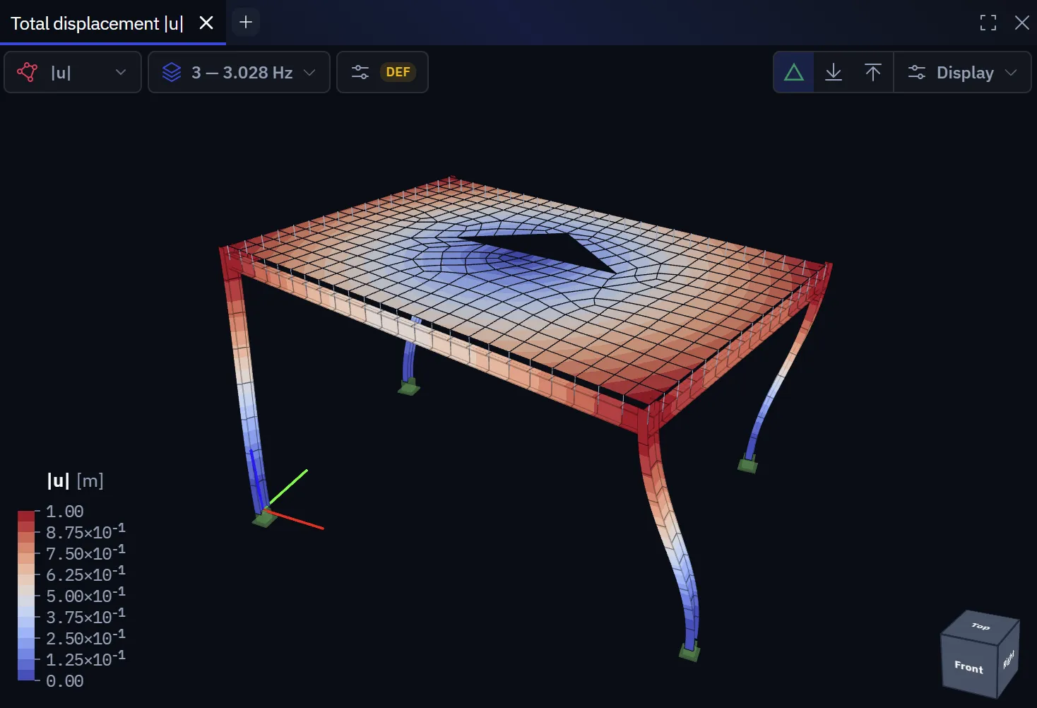
Surfaces read the same way. On a slab the mode shape is a contour of the scaled displacement, and the number that matters is the frequency beside it:
What the first modes usually tell you
| Symptom | Likely meaning |
|---|---|
| First mode very low (well under 1 Hz) in a building | The structure is much more flexible than intended. Check bracing and support restraints before believing it |
| First mode local rather than global | A single member or panel vibrating on its own. Often a modelling artefact, such as a member with mass but almost no restraint |
| Two nearly identical frequencies | A symmetric structure with modes in two directions, or a torsional mode close to a translational one. The latter matters for seismic behaviour |
Floor vibration
A floor's fundamental frequency should exceed about 4–5 Hz, or 8 Hz or more for rhythmic activity. That rule of thumb is a screening test, not a serviceability check. A proper assessment needs response factors and a damping assumption, which a modal analysis alone does not provide. Use the frequency to decide whether you need that assessment.
Limits in this release
- Frequencies come from the linear elastic, uncracked stiffness. For concrete, real frequencies are lower; codes give stiffness reductions for this.
- Damping is not part of the eigenvalue problem and is not modelled.
- Response spectrum and time-history analysis are not in this release. The modal result is the input they would need, not a substitute for them.
- Non-structural stiffness (cladding, partitions) is not modelled and typically raises real frequencies above the calculated ones.
Related
Linear buckling uses a closely related eigenvalue solution, and its mode shape can be fed to a second-order analysis as a §5.3.2(11) imperfection. Element formulations describes how mass is distributed within each element.
Something wrong or unclear on this page? Tell us, and it gets corrected.